Nets performance by star combo

In screencast #3, which builds on #2 , I plot the Nets team performance by the combination of stars that take the court in ‘21 NBA regular season.

code: https://gist.github.com/bhoung/769ea023915bc7f6802f667249b54508

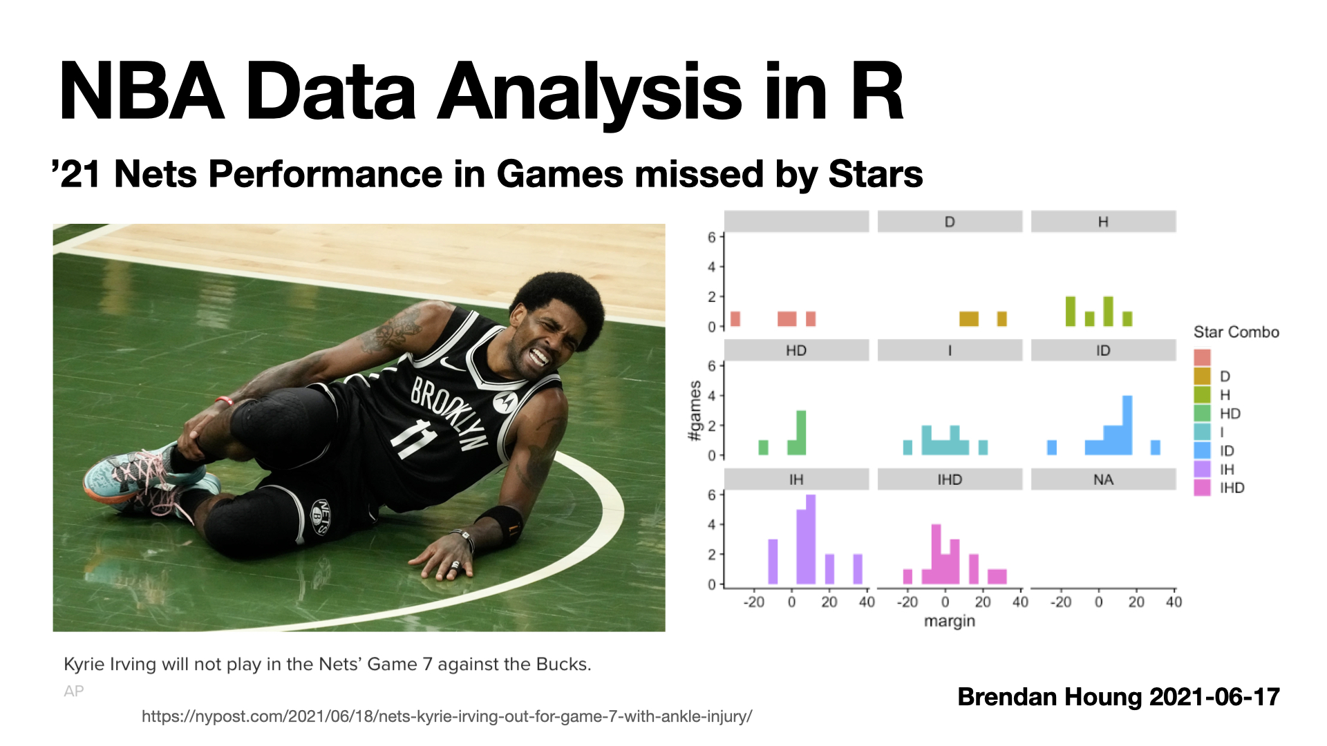
link to YouTube screencast #4 (2021-06-17) here

dfm %>% group_by(N_stars) %>% summarise(mean(diff), sd(diff), length(diff))

## # A tibble: 5 x 4
##   N_stars `mean(diff)` `sd(diff)` `length(diff)`
##     <int>        <dbl>      <dbl>          <int>
## 1       0        -6          17.0              4
## 2       1         2.44       13.8             18
## 3       2         7.43       12.5             35
## 4       3         2.93       13.1             15
## 5      NA        NA          NA                3

dfm %>% group_by(star_combo) %>% summarise(mean(diff), sd(diff), length(diff))

## # A tibble: 9 x 4
##   star_combo `mean(diff)` `sd(diff)` `length(diff)`
##   <chr>             <dbl>      <dbl>          <int>
## 1 ""               -6          17.0               4
## 2 "D"              19.7         9.29              3
## 3 "H"              -2.83       12.0               6
## 4 "HD"              1.8         8.53              5
## 5 "I"               0.222      12.6               9
## 6 "ID"              6.75       13.0              12
## 7 "IH"              9.44       13.0              18
## 8 "IHD"             2.93       13.1              15
## 9  <NA>            NA          NA                 3

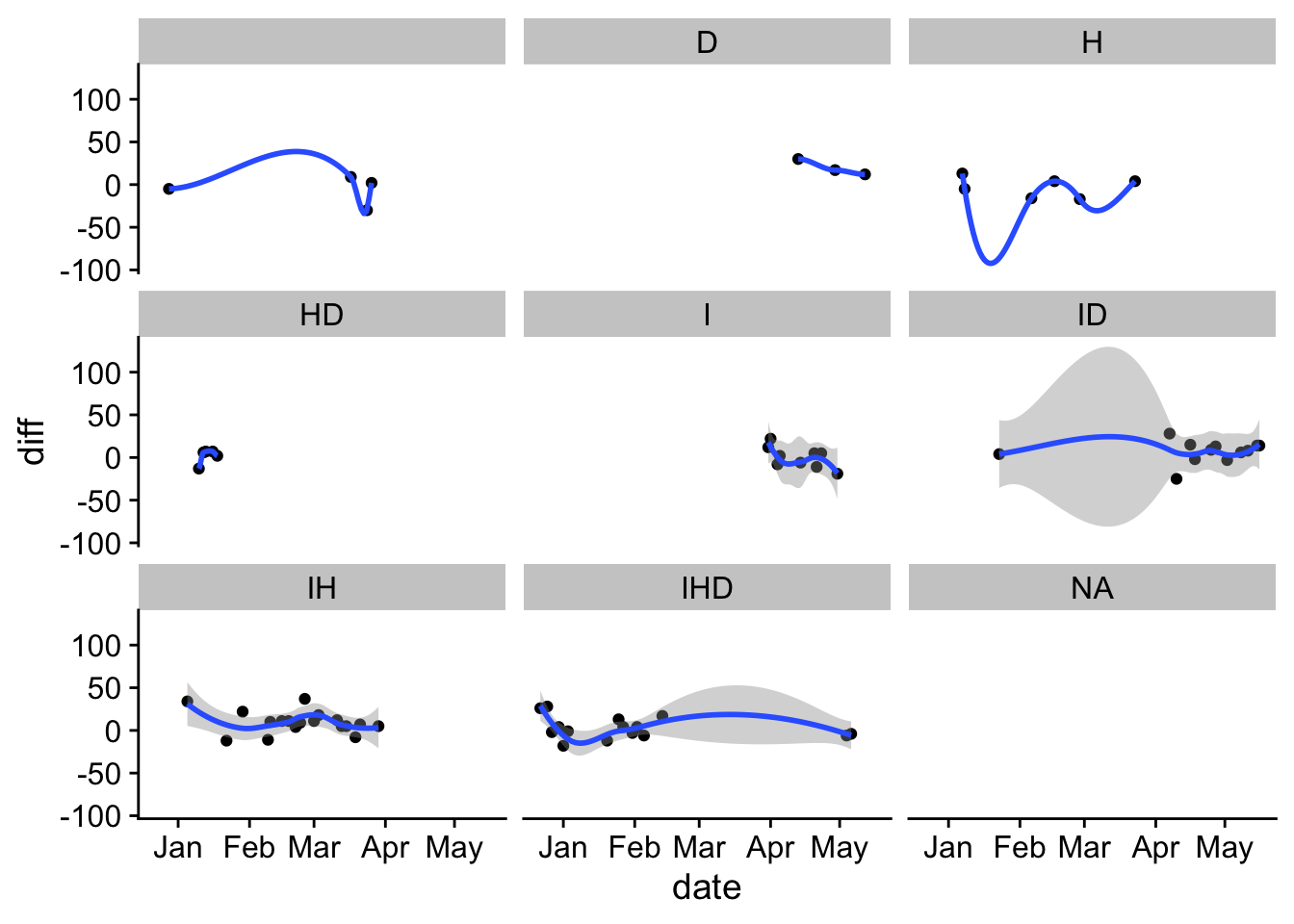
dfm %>% ggplot(.) + geom_point(aes(y=diff, x=date)) + facet_wrap(. ~ star_combo) + geom_smooth(aes(x=date, y=diff)) + theme_cowplot()

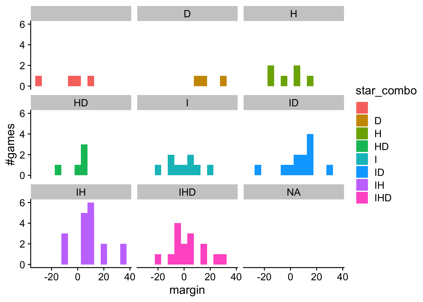
dfm %>% ggplot(.) + geom_histogram(aes(x=diff, fill=star_combo), binwidth = 5) + facet_wrap(. ~ star_combo) + theme_cowplot() + labs(x="margin", y="#games")

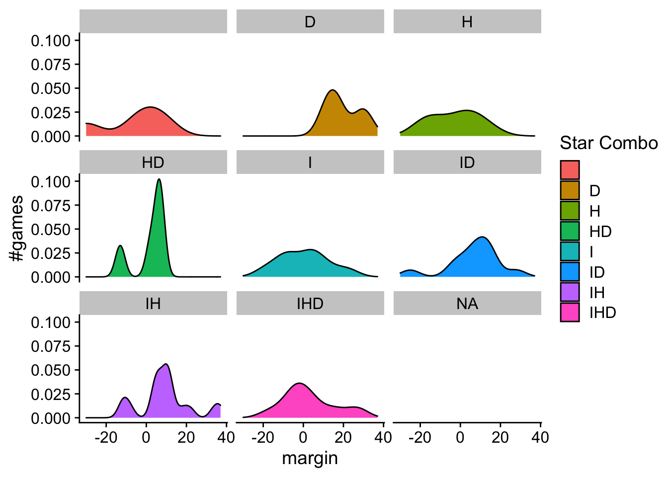
dfm %>% ggplot(.) + geom_density(aes(x=diff, fill=star_combo), binwidth = 5) + facet_wrap(. ~ star_combo) + theme_cowplot() + labs(x="margin", y="#games", fill="Star Combo")